In computer vision, a local feature is defined as "a small area that is significantly different from its immediate neighborhood," where "significantly different" can refer to many properties, such as brightness, color, texture, and so on. Sufficiently good features allow us to obtain more (semantic) information from an image beyond just color. For example, in a Convolutional Neural Network, features are extracted via convolutional kernels, and their hierarchical structure allows high-level information to be generated by combining low-level information. A network used for face recognition might contain neurons that perceive things like eyes, mouths, ears, hair, and skin, and use convolutional connections to excite units that perceive a face.

In this problem, we will study one of the most fundamental local features: "corners." Mathematically, a corner can be considered as the point where two edges intersect; an edge in an image can be thought of as a smooth, continuous segment on its gradient (derivative) image (if you draw a straight line on white paper with a black pen, because the black line is an area with width, there are actually two very close edges). Based on this consideration, the academic community has proposed several corner detection algorithms with certain performance, such as SUSAN, Harris, and CSS. We have provided some reading materials describing the SUSAN, Harris, and CSS algorithms, and your task is to select an algorithm suitable for yourself based on the provided materials and complete the corresponding implementation and optimization.

Note that in actual images, due to factors such as pixel discretization, color gradients, noise, and distortion, there are rarely well-defined edges. Therefore, these feature points found by certain mathematical methods are not necessarily corners from a human perspective, or they may have some deviations. However, in practical applications, although these detected points are not strictly corners, they usually still have sufficient features locally, so they are still widely used.

Input

The first line of the input contains two positive integers $w$ and $h$, representing the width and height of the image. It is guaranteed that $w \le 1280$ and $h \le 1280$.

The next $h \times w$ lines each contain $3$ non-negative integers describing a pixel. The three numbers in the $(i-1) \times w + j$-th line represent the RGB values (red, green, and blue) of the pixel at the $i$-th row and $j$-th column of the image. The integers are in the range $[0, 255]$.

Output

The first line contains an integer $k$, representing the number of detected corners.

The next $k$ lines each contain two non-negative integers $x$ and $y$, describing the coordinates of a corner. Note: In the coordinates, $x$ is the horizontal coordinate (width direction), and $y$ is the vertical coordinate (height direction). The coordinates of the pixel at the top-left corner of the image (row 1, column 1) are defined as (0, 0).

Examples

Input 1

(input data)

Output 1

(output data)

Note

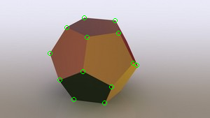
The image for this sample and its reference detection results are shown in the left and right images below, respectively.

Input 2

(input data)

Output 2

(output data)

Input 3

(input data)

Output 3

(output data)

Input 4

(input data)

Output 4

(output data)

Input 5

(input data)

Output 5

(output data)

Input 6

(input data)

Output 6

(output data)

Input 7

(input data)

Output 7

(output data)

Input 8

(input data)

Output 8

(output data)

Input 9

(input data)

Output 9

(output data)

Input 10

(input data)

Output 10

(output data)

Data and Scoring Method

There are a total of $20$ images in the test data, with each image being a test case. Additionally, there are $10$ images provided as your reference cases and pre-test data. Note that the pre-test data for this problem is exactly the same as the samples, and the evaluation results of the pre-test data have no relation to the final evaluation results.

We use the results of CSS + Harris (refine) as the reference algorithm and use the results manually labeled on the reference algorithm as the reference answer.

When evaluating whether your output corners are correct, we will perform a maximum bipartite matching between your output corners and the reference corners. If a pair of points $a$ and $b$ satisfies that $a$ is within a $5 \times 5$ range centered at $b$, then we consider this corner pair to be matchable. If one of your output corners is in the maximum matching, we consider that corner to be correct.

The score ratio for each test case is denoted by $F_1$, which is defined as:

$$ F_1 = \frac{2\mathit{TP}}{2\mathit{TP}+\mathit{FP}+\mathit{FN}} $$

where $\mathit{TP}$ (true positive) is the number of correctly output corners (i.e., the size of the maximum matching), $\mathit{FP}$ (false positive) is the number of incorrect corners in your output, and $\mathit{FN}$ (false negative) is the number of correct corners that were not matched by your output.

Further explanation of $F_1$: The proportion of correct points in your output, $\frac{\mathit{TP}}{\mathit{TP}+\mathit{FP}}$, is called "precision"; the proportion of points that should have been output that were captured by your output, $\frac{\mathit{TP}}{\mathit{TP}+\mathit{FN}}$, is called "recall." $F_1$ is the harmonic mean of precision and recall.

The images we selected ensure that the algorithms in the provided materials will have good performance under specific optimizations. For the given test images, the $F_1$ detection rate of the reference algorithm for corners is around $90\% \sim 100\%$.

Implementation Details

In addition to the reference cases, the provided files contain two types of files: documents describing the reference algorithm and some of its implementations, and some tools. You may use these materials as you wish, including reading and implementing them, using parts of the code directly, or using them to assist your implementation or debugging. You may also choose not to use them and complete this problem entirely on your own.

We recommend that you implement one or two of the three algorithms provided in the materials and attempt your own adjustments or modifications based on them. The implementation difficulty and effectiveness of the three algorithms, from low to high, are: SUSAN (or one of its implementations, FAST), Harris, and CSS.

The tools include: a conversion tool between input and PNG format images, and a visualization tool for the output results.

For the specific usage of the provided files and a guide to the documentation, please read README.pdf in the files.

Finally, please note: If you need to use the code from the provided files, you should copy it directly into your submitted code; you should not attempt to include it using methods like #include. You can only submit one file, and the testing environment will not be able to read these provided files.